Pystan – The model, differences between two groups

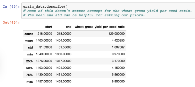
In the last post we talked about the data set up and writing the model for comparing crop yields from two different counties in England.

This will run the model for us.

# Compiling and producing posterior samples from the model.
fit_compare_groups = pystan.stan(model_code=model_string, data=compare_groups,
 iter=1000, chains=4)

And now we can look at the model output.

fit_compare_groups
<pre>Inference for Stan model: anon_model_1f0ebaa1784e353e9595dea46e6ad140.
4 chains, each with iter=1000; warmup=500; thin=1; 
post-warmup draws per chain=500, total post-warmup draws=2000.

           mean se_mean     sd   2.5%    25%    50%    75%  97.5%  n_eff   Rhat
mu[0]      5.44  3.4e-3   0.15   5.14   5.34   5.44   5.55   5.74   2000    1.0
mu[1]      3.08  2.5e-3   0.11   2.86   3.01   3.08   3.16    3.3   1930    1.0
sigma[0]   1.31  2.4e-3   0.11   1.11   1.23   1.31   1.38   1.54   2000    1.0
sigma[1]    0.8  1.8e-3   0.08   0.66   0.74   0.79   0.85   0.96   1974    1.0
lp__     -70.59    0.04   1.37  -74.0  -71.3  -70.3 -69.57 -68.82   1092    1.0

Samples were drawn using NUTS at Wed Jul  5 12:42:43 2017.
For each parameter, n_eff is a crude measure of effective sample size,
and Rhat is the potential scale reduction factor on split chains (at 
convergence, Rhat=1).

Right off the we can that mu0 and mu1 are not the same. A few lines of code will help verify this.

# Plotting the posterior distribution
fit_compare_groups.plot()

This is the trace plot from the model.

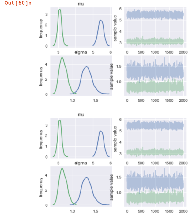
There are a few other things you can do as well.

# Returns the mean of the location paramter mu
mu = fit_compare_groups.extract(permuted=True)['mu']
np.mean(mu, axis=0)

and

mu_df = pd.DataFrame(mu)
mu_df.columns = ['mu0', 'mu1']

# The probability that mu0 is smaller than mu1
l = mu_df.mu0 < mu_df.mu1
sum(l)/len(l)

Pystan – Setup, differences between two groups

Often I stumbled across data where I am looking at two groups of things. In some of our recent work our group was looking at bacteria found in caves and bacteria found above ground. Granted there is a lot more going on then just surface and subsurface stuff. It’s actually better to wrap this all up in something called a hierarchal model.

But it’s useful to look at just a simple two group problem.

I like to either simulate some fake data or grab a data set from outside my field. In this case I stumbled across Three centuries of English grain yields Grain yield database .

I picked two counties in England that look neat.

import pystan
import pandas as pd
import matplotlib.pyplot as plt
import seaborn as sns; sns.set_context('notebook')
from IPython.display import Image
import numpy as np
%matplotlib inline

 

Berkshire

Hampshire

 

maps by Unknown (wikimedia), distributed Creative Commons Attribution-Share Alike 3.0 Unported

# Import data
grain_data = pd.read_csv('./three_centuries_of_grain/berkshire_hampshire_grain_1349_1458.txt', sep="\t")

A quick exploratory plot using the seaborn package.

Well, a few things stand out. First, the two grain yields look different. Second, it’s non-linear. I would guess you would get a better fit using splines or state-space model. That’s for a later post.

# And here we just look at the bulk difference between Hampsire and Berkshire
sns_plot = sns.stripplot(x="County", y="wheat_gross_yield_per_seed_ratio", data=grain_data);

Now we get this wrangled into something pystan can use.

# We seperate out each county into it's own data frame.
berkshire = matched_grain.loc[matched_grain['County'] == 'Berkshire']
hampshire = matched_grain.loc[matched_grain['County'] == 'Hampshire']

# Here is the data to model. Note we convert the dataframe column to a python list.
y1 = berkshire.wheat_gross_yield_per_seed_ratio.tolist()
y2 = hampshire.wheat_gross_yield_per_seed_ratio.tolist()
# Here we just ask what is the length of the data.
n1 = len(y1)
n2 = len(y2)

# Dictionary containing all data to be passed to STAN
compare_groups = {'y1': y1,'y2': y2,'N':[n1,n2]}

The Stan model

# Corrected by Bob Carpenter
model_string = """
data {
int N[2];
vector[N[1]] y1;
vector[N[2]] y2;
}
parameters {
vector[2] mu;
vector<lower=0>[2] sigma;
}
model {
mu ~ normal(0, 10);
sigma ~ cauchy(0, 5);
y1 ~ normal(mu[1], sigma[1]);
y2 ~ normal(mu[2], sigma[2]);
}
"""

Best practices would be to store this model in a stan model and then load it in. But for playing around this is ok.

 

The full jupyter notebook using python and pstan is here on my github account.

 

Pystan musings

One of my (our?) recent shifts in the past few years is moving towards a full Bayesian framework for carrying out our work. This required (and still requires) a pretty big shift in how we think about our data.

1. Embrace uncertainty and noise in the data.
2. Directly model the data (no permanova or t-test anymore).
3. Write models from scratch using pystan and the jupyter notebook.

To this end I have a github repo set up where I am dumping out me working through pystan with examples from a range of disciplines.

Winter Pystan Musings

I’ll talk about the models and such in a later post.

 

Scratch spaces

I get torn between putting out work here, on github and on google+ . I think each site serves a slightly different purpose. Github for code, google+ for a narrower audience, and here maybe for a scratch space for writing about processes.

 

 

Primers working!!!

So I am wrangling with getting these literature based PKS I primers working for my PhD project. Finally success!!!

PKS I Primers

degKS2F 5’-GCIATGGAYCCICARCARMGIVT 

degKS2R 5’- GTICCIGTICCRTGISCYTCIAC

760 bp fragment

Schirmer, A., R. Gadkari, C. D. Reeves, F. Ibrahim, E. F. DeLong, and C. R. Hutchinson. 2005. Metagenomic analysis reveals diverse polyketide synthase gene clusters in microorganisms associated with the marine sponge Discodermia dissoluta. Appl Environ Microbiol 71:4840-4849.

Master mix for one reaction (bring up to 15 uL total with DNA and water)

in uL

H2O 6.00

PCR Buffer 1.5

DNTP 1.5

BAS 0.14

Primers 0.15 each

Taq 0.1

MgCl 2.4

DMSO 1.4 ***I typically don’t use DMSO so swap in water here)

GEL!!!! The first well in each line is the positive control

 

Returned from Parashants

Just got back from an amazing time in the Parashants! Will post an update shortly.

Figshare – GC content compared to genome size

For those that are interested in opensource science I am over on figshare as well.

Just posted GC content and genome size plot from some data I mined from NCBI awhile back.

http://figshare.com/articles/GC_Content_vs_Genome_Size_of_4231_Bacteria_Genomes/97275

 

 

I like this sketch I did. This shows the spatial relationship between several cave pools in cross section to the geologic structures in the area. The numbers with the arrows are the strikes of the flowstone and rimstone dams.

The circle in the lower right is an equal hemisphere projection. The lines are best thought of as planes sitting inside a hollow hemisphere. This is one way to represent different geologic features as planes.

Optimizing PCR reactions for gene amplification Part II

Here is a slightly modified one for those troublesome genes that won’t amplify or if you get lots of smearing.

Basic Master Mix recipe for AmpliTAQ gold

for 15 µL reaction

(volumes in µL)
H2O 9.57
10x PCR Buffer 1.5
100x BSA 0.125
Forward Primer 0.1
Reverse Primer 0.1
TAQ 0.15
MgCl2 1.5
DMSO 1.5

Trees! and some field work

I’ve been working on this thing here

This shows the effect of different alignment programs on the same 16S data set.
Pretty neat.

I am going out on Saturday to the Ojito Wilderness area to do a strat section on a mesa. I want to show folks what a geosciences notebook looks like.

Sunday will be some data from Lechuguilla Cave (one of the places I work in)